
Enough talk; let's move to the first concept: Epochs, or the number of iterations. In earlier chapters, we said that model fitting is essentially performing gradient descent at the same scale many times. Epochs represent how many of those gradient descents you want in one training run. In Machine Learning, hyperparameter values need to be adjusted for the situation. Hyperparameters directly affect the results of your model's training.
The second concept: Random Forests. This is an algorithm I personally loved using in competitions (of course, the version I used was much more complex than the one I am teaching). Since this thing works so well, it goes without saying that it needs a lot of computing power. Next, let's explain why it needs that power:
If we draw a Random Forest, it roughly looks like this:
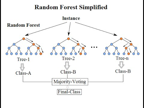
At its core, a Random Forest is a kind of "pooling of ideas": multiple decision trees give their own votes, and the result of the votes is used to determine the value of a question.
Where exactly is the randomness in a Random Forest? To answer that, we need to return to how a Random Forest keeps every tree different. There are two factors.
First, each tree, within the dataset,randomlydraws a training set for training. Notice that I highlighted this word, random. That is why the word matters.
Second, when a tree splits at a node, it uses only some of the features to make the split. What does this mean? For example, if a dataset has 9 features in total, we usually use (features)^1/2 features. When the algorithm reaches a node, it has to consider which feature to use. This is where the square root of 9 = 3 from earlier becomes useful. The algorithm fits on the randomly obtained data group, finds the best (optimal) feature, and finally makes the split.
Another crucial hyperparameter in Random Forest is Max Depth. Max Depth means the maximum number of nodes this tree can have. If this hyperparameter is made large, the computing requirement is high; if it is made small, the model may not fit well. So we usually choose a fairly suitable value.
After all the trees make their final judgments, we gather the results and make one final decision.
That is roughly the idea of Random Forest.
Next is an advanced algorithm related to Random Forest: the Boost algorithm. Here we will explain what I personally think is the best algorithm in the boost family, XGBoost.
First, we need to understand what the Boost algorithm actually is.
The Boost algorithm is essentially multiple models arranged in a sequence. First train model one and get its result, then train model two and get a (perhaps) better result, then train models 3, 4, 5, 6, and 7, and so on. The Boost algorithm was born for extreme performance.
If the Random Forest algorithm is for preventing overfitting, then the Boost algorithm is for preventing underfitting.
We can compare the Boost family of algorithms to a "top student's growth diary."
Usually, the model at sequence one is relatively weak. Its Max_Depth is usually small, generally 1, which means one split.
We usually call model 1 a "weak learner." For example, suppose we feed model 1 ten thousand math problems worth one point each. If model 1 gets six thousand right and four thousand wrong, we focus on those four thousand wrong problems and give them higher scores, such as two points. Then we feed them together with the six thousand correct problems to model 2, which has a higher Max Depth. Model 2 will naturally think, "Oh, each of these problems is worth two points," so the rewards and penalties are clearer. Getting a two-point problem wrong is more serious than getting a one-point problem wrong.
Model 2 will then focus on solving the two-point problems, because it wants more rewards and does not want to receive a severe penalty for getting a two-point problem wrong.
Model 2 will also have things it cannot solve. For example, it may get eight thousand questions right and two thousand wrong. We then give those two thousand questions (for example) four points, and model 3 will treat those high-value questions the way model 2 treated the two-point questions.
Here I will add a picture to describe this process:
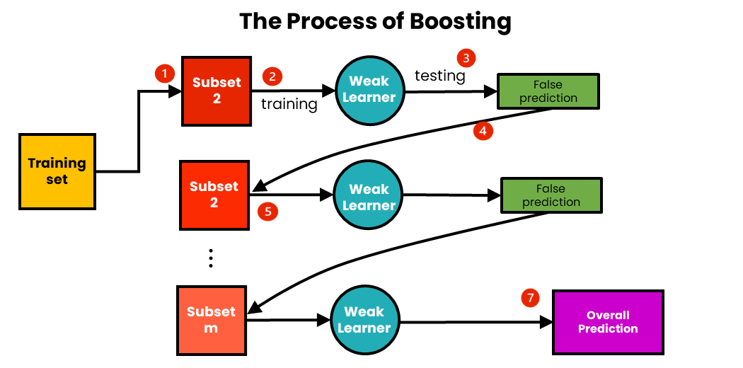
When our series of models (usually four to six, to prevent overfitting) has finished training, we next evaluate the report card submitted by the models. We give a higher weight to models with better results (fewer wrong answers), and the opposite to models with more wrong answers. When we need to solve a problem, it is like a seminar: we let these models share their ideas. A model with a higher weight has more say, speaks more boldly and loudly, and our final result naturally listens to it more. The opposite is true for a low-weight model; we use its opinion only a little.
That is the principle of Boosting. Next we will add the mathematical explanation. If math is not your strength, you can skip this part and go straight to the next section.
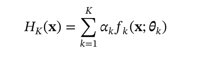
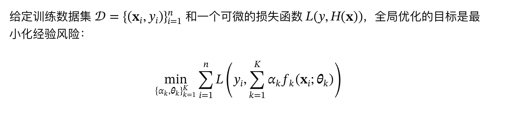
That is roughly the mathematical explanation of Boosting. This actually involves a greedy algorithm, which we will explain later in the final few chapters of Machine Learning, and even when we discuss LLMs.
Next, we will introduce the two most widespread schools of Boosting:
1.Ada Boost
So what is AdaBoost? As its name suggests, it means Adaptive Boost, an adaptive Boost algorithm.
The essence of the Ada algorithm is that it does not require us to adjust thescoreshyperparameter every time a model finishes training. The algorithm assigns the scores to the models automatically.
The advantage is convenience: it is very hands-off, so it is suitable for letting the algorithm train on its own without someone needing to manage it.
2.GBDT
GBDT, whose Chinese name is Gradient Boosting Decision Tree. In GBDT, we do not make every model work through all ten thousand questions. We focus on having the model study the four thousand wrong questions. We ask it to guess what was wrong with those four thousand questions and what the difference was. For example, a person is 180 tall, model 1 guesses 150, a difference of 30; model 2 guesses the difference is 20, gets it wrong again, and passes it to model 3; model 3 guesses model 2's difference is 9; and so on;
In the end, we add together the differences obtained by all the models, bringing us very close to the real answer. This is called GBDT.
I suddenly realized that this chapter only talks about algorithms and is a little mathematical. Since that is the case, let's put XGBoost aside for now and talk about Matplotlib first. Of course, the XGBoost chapter has already been recorded and will come after Matplotlib. The next one, Matplotlib, is a big project, so look forward to it~
See you in the next chapter!
References & image sources:
1. NVIDIA glossary
https://www.nvidia.cn/glossary/xgboost/
2. Figure 2 (Boost Algorithm):
https://medium.com/@brijesh_soni/understanding-boosting-in-machine-learning-a-comprehensive-guide-bdeaa1167a6
3. Figure 1 (Random Forest Simplified):
https://williamkoehrsen.medium.com/random-forest-simple-explanation-377895a60d2d