Learning rate is a Hyper Parameter, abbreviated here as HP, or hyperparameter. HP is a parameter decided before ML begins, and it can directly affect the numerical value of ML performance. Other HPs include Context Window (LLM), random level, and learning rate. Notice that while learning the basic concepts here, we must distinguish one concept: ordinary Parameters, or parameters. Ordinary P is simply the result after ML learns. Here, we are more inclined to call the results of training LLM, VLM, and ALM-type Gen AI the result. Ordinary ML, such as Linear Fit, does not involve Parameters.
Let's return to Learning rate. LR is simply the size of the jump a Machine makes while learning. Compare it to running: when you run, the larger your stride, the fewer steps you need to cover a distance. The opposite is also true. But LR is not better when it is larger. LR needs a relatively suitable value. Here is a table for reference (it does not apply to every situation).
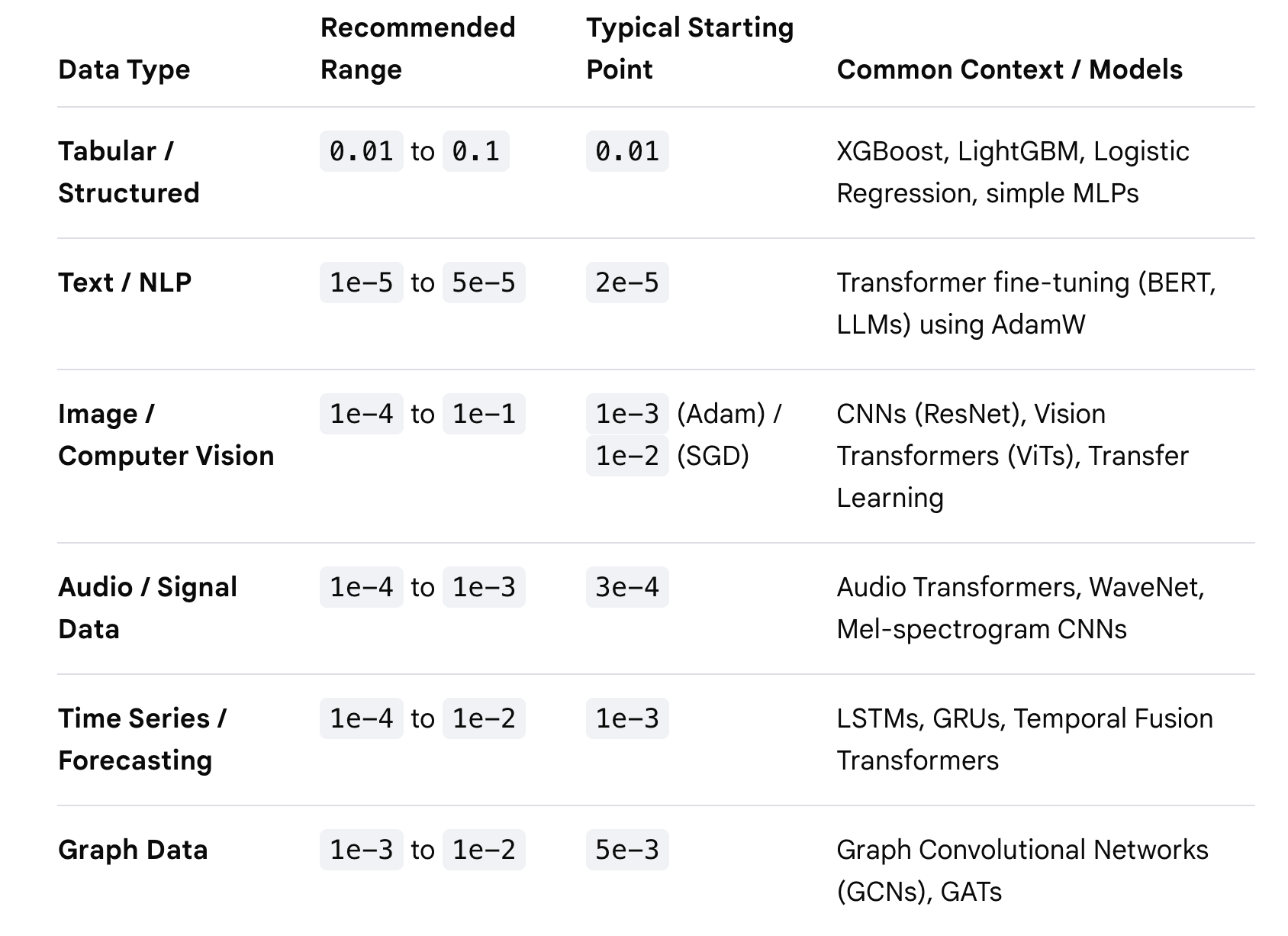
There are quite a few concepts involved here, so I will not explain them one by one; progress comes first.
Now that LR has been introduced, we officially enter SciKit Learn.
The classic Import section as usual:
Let's start with the simplest Linear regression here.
import numpy as np
from sklearn.linear_model import LinearRegression

X = np.array([1, 2, 3, 4, 5]).reshape(-1, 1)
# A random array

y = np.array([30000, 42000, 51000, 68000, 75000])

model = LinearRegression()
# Call this model

model.fit(X, y)
# Start fitting

slope = model.coef_[0]
intercept = model.intercept_

You can directlyprintprint it now.
So we have simply completed a Linear regression Fit. Next, we will use Logistic Regression to go a step further.
import numpy as np
from sklearn.model_selection import train_test_split
from sklearn.linear_model import LogisticRegression
from sklearn.preprocessing import StandardScaler


Still, just some arbitrary arrays
X = np.array([, [2, 3], [3, 8], [24, 25], [30, 28], [12, 18],
, [36, 30], [18, 22], [6, 12], [40, 35], [10, 6]
])
y = np.array([0, 0, 0, 1, 1, 1, 0, 1, 1, 0, 1, 0])

Here we introduce Train test split, a very useful array-splitting tool
X_train, X_test, y_train, y_test = train_test_split(X, y, test_size=0.3, random_state=42)

We scale X and y (turning them into [0,1]]-type values)
scaler = StandardScaler()
X_train_scaled = scaler.fit_transform(X_train)
X_test_scaled = scaler.transform(X_test)

Fit
model = LogisticRegression()
model.fit(X_train_scaled, y_train)

y_pred = model.predict(X_test_scaled)
This is the ultimate boss of this chapter: the SGD model.
In the pure theory of the previous chapter, we introduced Gradient descent. Now let's make it real with SK learn's SGD model.
import numpy as np
from sklearn.linear_model import SGDClassifier
from sklearn.preprocessing import StandardScaler
from sklearn.model_selection import train_test_split

No explanation here.
X = np.random.randn(200, 4)
y = np.random.randint(0, 2, size=200)

X_train, X_test, y_train, y_test = train_test_split(X, y, test_size=0.2, random_state=42)

Scale the dataset first. In fact, scaling here can make the model structure more accurate.

scaler = StandardScaler()
X_train_scaled = scaler.fit_transform(X_train)
X_test_scaled = scaler.transform(X_test)

Introduce the model
model = SGDClassifier(
    loss='log_loss',
    learning_rate='adaptive',
    eta0=0.01,
    max_iter=1000,
    n_iter_no_change=5,
    random_state=42
)

Fit it
model.fit(X_train_scaled, y_train)
Notice that there is actually one more step after this (evaluating the model). I will not write it here for now; a separate chapter will later cover matplotlib and model evaluations.
With that, we have completed one Logistic Regression (logistic regression).
I apologize here: I got the chapter order a little mixed up and left out an important concept (Random Forests).
So this SK learn chapter will not fit a random forest for now. Sorry.
That is roughly the content of this chapter. In fact, opening a whole chapter to talk about SK learn is a very difficult topic, because without introducing some more advanced content, there is not much content about SK learn by itself.
Next time we will focus on introducing Random Forests and matplotlib. I hope everyone is happy every day. Goodbye!