
Let's start with Linear Regression. Simply put, Linear Regression connects scattered spots on a chart into a line, whether it is a straight line, Hyperbola, Quadratic Functions, or any line with a pattern. From this, we can build a Model to Predict some values.
For some specific applications, here are a few examples:
Finance and real estate: analyze how house size, location, and other factors affect house prices or forecast trends in stock prices, currency exchange rates, and market returns.
Marketing and business: evaluate the actual effect of advertising spend (the independent variable) on sales (the dependent variable), and analyze market share and customer lifetime value.
Medicine and health: study the quantitative relationship between risk factors such as blood pressure, cholesterol, and age and disease development trends or a patient's recovery period.
Operations and production management: use historical data to predict future electricity consumption, logistics transportation time, or industrial production output
and other examples. So how exactly do we carry out this process? We need to introduce a Concept - Lost Function,as shown below:
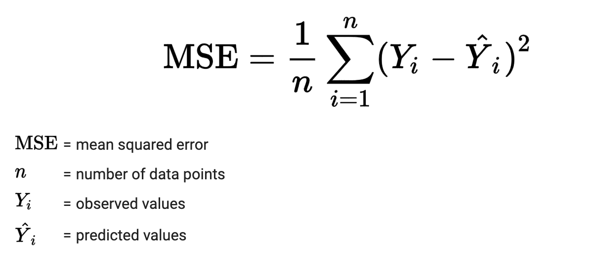
The larger the MSE value, the less precise the Model is, so we need to lower the MSE value as much as possible. Humans can easily use the least squares method to find a very precise value, but a machine is not a human; it only knows 0 and 1. We can use Python to solve this problem.
First, let's see how the value of K is calculated.
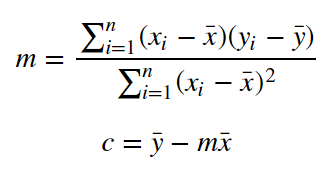
So how do we let the machine calculate it? We do not need to stubbornly write out every formula like competition Python. We can borrow some tools from Numpy, such as Vstack. The implementation is as follows:
import numpy as np

Make an arbitrary Array
x = np.array([1, 2, 3, 4, 5])
y = np.array([2.1, 3.9, 6.2, 8.1, 10.2])

Implement it with Vstack
A = np.vstack([x, np.ones(len(x))]).T


solution, residuals, rank, singular_values = np.linalg.lstsq(A, y, rcond=None)

slope, intercept = solution
print(f"Slope: {slope:.4f}, Intercept: {intercept:.4f}")
This method is relatively precise, but is there an even more precise method? This brings us to Gradient Descent.
Using the picture below, we can quickly understand what GS is actually doing.
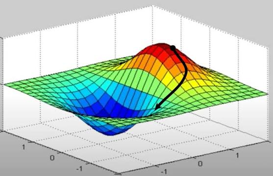
Here, the X and Y axes are the values of K and B in y=kx+b. Gradient descent adjusts these values to make the Z axis (the lost function, which is the MSE value) as small as possible. As shown, the lowest valley in the blue area is the value we are looking for.
As with the least squares method, we do not need to build complicated formulas to calculate it. We can leave that to the machine and use some tools.
Here we need to introduce the concept of Learning rate. Simply understood, it is the rate/speed of machine learning. We need to adjust this value precisely to make the machine learn as well as possible. Notice this Basic concept: Learning rate is actually a Hyper Parameter (hyperparameter), which we will mention again later.
We will also briefly pass over the mathematical principle here with a picture:
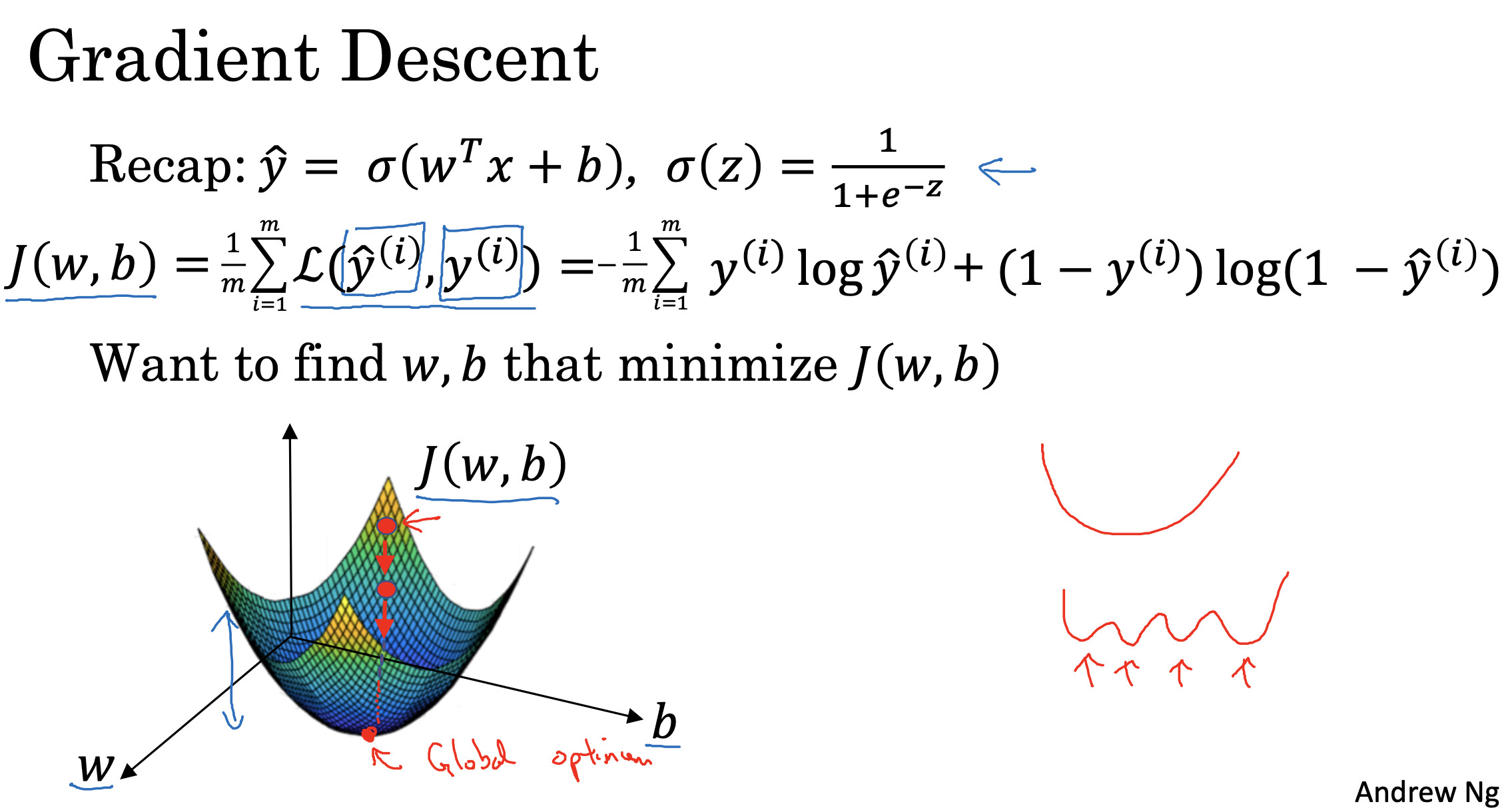
For this code, we need to learn deeper content (SK learn) before we encounter it, so we will meet this code in the next chapter.
That is roughly all the content of this chapter. It is actually rather difficult to understand, so everyone can refer to some YouTube lessons to deepen their understanding.
That is all for this episode. See you next time!