Advanced NumPy and Basic Pandas

Do you remember that I mentioned several ways to obtain data last time? This time we will begin with importing Csv Files.

Open a new Code Cell in Colab

import pandas as pd

file = pd.read_csv('/content/files/test')   # Fill in the file directory between the green single quotes here

With that, we have successfully imported a csv file. A Csv file imported by Pandas roughly looks like this in the Colab terminal:

Notice this small tip: in Colab, most files, variables, and arrays do not need print(), like this:

file

Run this cell with the button on the left, and the result printed will look like the picture below:

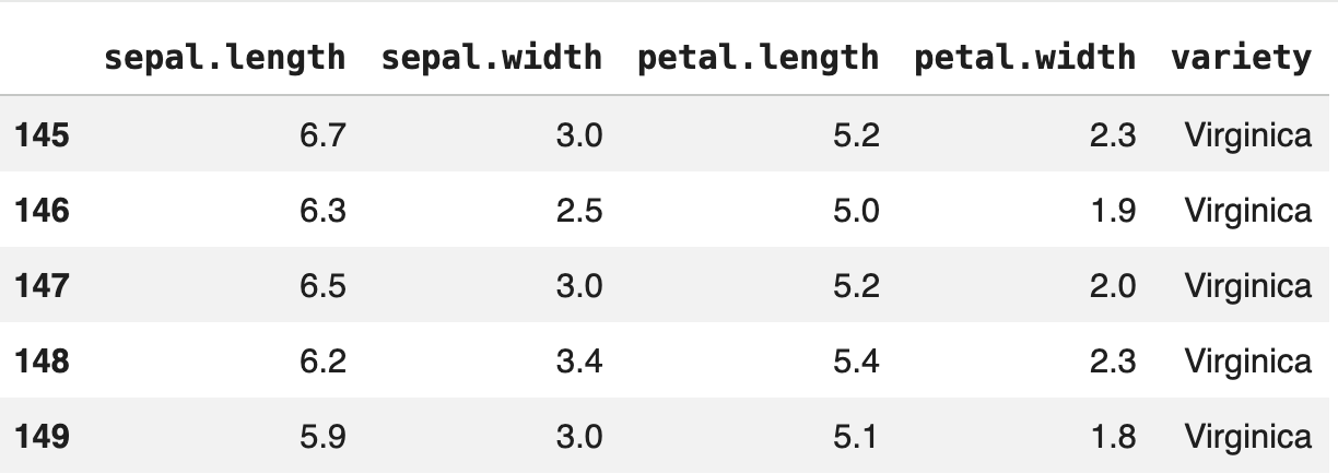
(Notice that this picture shows only part of it)

Here is another way to import a file without attaching Drive:

There is no explanation here; you can just copy the answer:

from pathlib import path
import pandas as pd

path = Path("folder") / "subfolder" / "file.txt"

file = pd.read_csv('path')

This lets Pandas read a csv file without depending on the connection between Google Drive and Colab.

Last time we explained Numpy's Array. As its higher-level replacement, Pandas also has a similar data store: the Pandas DataFrame, abbreviated df. Built on the Numpy Array, it makes computation faster and is easier to use.

import pandas as pd

files = pd.read_csv('/content/ml-ds/test')

df = pd.DataFrame(files)

With that, a simple DF has been created.

Next, let's look at some basic uses of a Pandas DF

import pandas as pd

files = pd.read_csv('/content/ml-ds/test')

df = pd.DataFrame(files)

View the first five rows:
df.head()

View the last five rows:
df.tail()

View a specific column in a row:
df.loc[0,"sepal_length"]
Format: dataframe name.loc[row number, "column name"]

View one column across all rows:
df.loc[: , "sepal_length"]

View the content within a range of rows/columns:
df.loc[1:3, "sepal_length":"petal_length"]

iloc and loc do not have a significant difference in function. iloc only does not rely on the column index name when retrieving a column; it uses the column index number instead, for example:

df.iloc[0:2, 6:8]

These are some less common uses. Now let's introduce some common ones:

import pandas as pd

files = pd.read_csv('/content/ml-ds/test')

df = pd.DataFrame(files)

View all rows for one index name:
df["proximity"]

Filter by a condition:
df["proximity"] == "island"

Sort a Column by size:

df[df["ocean_proximity"] == "island"].sort_values("median_income", ascending=False).head(10)

After the Pnadas indexing techniques above, let's explain some Pandas data-cleaning techniques:

import pandas as pd

files = pd.read_csv('/content/ml-ds/test')

df = pd.DataFrame(files)

Example of removing duplicates:
df.drop_duplicates(inplace=True)

Remove N/A-type data
df.dropna(subset=['critical_column'], inplace=True)

Fill in blank data (using median here):
median_value = df['numeric_col'].median()
df['numeric_col'].fillna(median_value, inplace=True)

Sum up an entire column:
df['Total'] = df.sum(axis=1, numeric_only=True)

Sum multiple Columns:
df['Total'] = df[['Column_A', 'Column_B']].sum(axis=1)
Or:
df['Total'] = df.iloc[:, 0:3].sum(axis=1)

Here, most basic uses of Pandas have basically been covered. This episode was updated after I finished updating Chapter 4, so I finally caught up. If anything is missing, please email me with advice at the bottom of the main site. Thank you.

That is basically all the content of this chapter. Recently I have mainly been studying deeper Deep learning, mostly about Computer Vision, such as Ultrlytics and OpenCV. Later I will also produce several episodes of Deep Learning content, not limited to ML frameworks. Here is a preview: after Linear regression&gradient descent comes Scikit- Learn, and after that we basically enter Model Building. Then there will be tutorials on matplotlib and Seaborn (mostly charting), followed by Transformers. After Transformers we enter the field of Deep Learning, and finally I will give a light lesson on small-parameter LLMs (SLMs) under the Transformers framework. You can look forward to it. See you next time～

记得上期我提到了获取数据的几种方法吗，这期我们就以导入Csv Files开头。

在Colab新开一个Code Cell

import pandas as pd

file = pd.read_csv('/content/files/test')   #这里绿色单引号中间填文件的directory

这样，我们就成功的导入了一个csv文件。Pandas导入的Csv文件在Colab的terminal中大概长这样：

注意这里有个小tips，在Colab里面，大部分文件，variables，array都是可以不需要print（）的，像这样：

file

左边按钮运行这个cell，就会有如下图一般打印出来的结果：

（注意这张图只截取了部分）

这里再教大家一个不需要外挂Drive也能导入文件的办法：

这里就不解释了，抄答案即可:

from pathlib import path
import pandas as pd

path = Path("folder") / "subfolder" / "file.txt"

file = pd.read_csv('path')

这样可以通过Pandas读取一个csv文件,而且不需要依赖Google Drive和Colab的联动。

上期讲解了Numpy的Array，那么Pandas作为他的上位替代，也拥有一个类似的数据存储，就是Pandas DataFrame，简称df。在Numpy Array的基础上，增快了运算速度，而且更加好用。

import pandas as pd

files = pd.read_csv('/content/ml-ds/test')

df = pd.DataFrame(files)

这样，一个简单的DF就已经被建立了。

接下来，我们来看一些基础的Pandas DF的基础用

import pandas as pd

files = pd.read_csv('/content/ml-ds/test')

df = pd.DataFrame(files)

查看前五行：
df.head()

查看最后五行：
df.tail()

查看某一行的某个特定的column：
df.loc[0,"sepal_length"]
格式：dataframe name.loc[row number, "column name"]

查看所有row里面的某一个column：
df.loc[: , "sepal_length"]

查看某一个范围的row/column内的内容：
df.loc[1:3, "sepal_length":"petal_length"]

iloc和loc在功能上并没有显著区别，只是iloc对于从于column的检索不依赖column index name，而是column index number，例如：

df.iloc[0:2, 6:8]

这些是一些较为不常用的用法，现在来介绍一些常用的：

import pandas as pd

files = pd.read_csv('/content/ml-ds/test')

df = pd.DataFrame(files)

查看某一个index name的所有row：
df["proximity"]

筛选某一条件：
df["proximity"] == "island"

排序某一个Column的大小：

df[df["ocean_proximity"] == "island"].sort_values("median_income", ascending=False).head(10)

上面讲完了Pnadas的索引技巧，现在来讲解一些Pandas的清洗数据技巧：

import pandas as pd

files = pd.read_csv('/content/ml-ds/test')

df = pd.DataFrame(files)

去掉重复的例子：
df.drop_duplicates(inplace=True)

去掉N/A类型数据
df.dropna(subset=['critical_column'], inplace=True)

填入空白数据（这里使用median填入）：
median_value = df['numeric_col'].median()
df['numeric_col'].fillna(median_value, inplace=True)

Sum up一整个列：
df['Total'] = df.sum(axis=1, numeric_only=True)

Sum多个Columns：
df['Total'] = df[['Column_A', 'Column_B']].sum(axis=1)
或者：
df['Total'] = df.iloc[:, 0:3].sum(axis=1)

这里，基本上大部分的Pandas基础用法都已经讲述完了，这一期是在我更新完Chapter4之后更新的，总算是赶完了。如有遗漏，请发邮件指教，在主站的最底下，感谢。

那么这基本上就是这一章节所有的内容了，最近我基本上都在学习更加深层的Deep learning，基本上是关于Computer Vision，例如Ultrlytics和OpenCV，以后我也会出几期Deep Learning的内容，而不仅限于ML的框架了，这里做个预告：Linear regression&gradient descent后是Scikit- Learn，再之后就基本上进入Model Building了，之后有matplotlib和Seaborn（基本上是图表化）的教程，再之后是Transformers，Transformers之后就进入Deep Learning的范畴了，最后浅浅的教学一下Transformers框架下的小参数LLM(SLM)。可以期待一波，大家下期见～